Optimal Output

Now that we understand the basis of fixed and variable inputs, we can start to do marginal analysis. Marginal revenue is the change in revenue generated by an additional unit of

output; when we get to graphing, it’ll also be the slope of the revenue curve. Marginal cost is the change in cost generated by an additional unit of output.

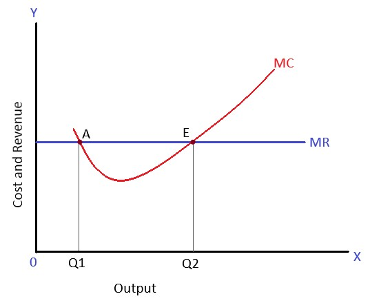
To maximize profits, firms follow the optimal output rule, which states that firms maximize profits when marginal revenue is equal to marginal cost. But the question you should be asking yourself is why? Well, that’s where cost curves – which will help you understand the rule graphically – come into play.

Source: Hamro Library

Q2 is the profit-maximizing quantity of output. At every quantity less than Q2, the additional revenue gained from producing the last unit is greater than the additional cost taken on. After Q2, the additional cost attained is greater than the additional revenue, decreasing profit. It’s very similar to the optimal consumption rule, which we covered much earlier.

More on that later, but here are some more terms to know for now. Marginal product or marginal physical product is the change in total output generated by an additional unit of input. Generally, this input is labor. Marginal revenue product is the dollar value of the change in output generated by an additional unit of input. You can also think of it as a marginal product multiplied by marginal revenue.

Because there are diminishing returns to inputs (you don’t want “too many cooks in the kitchen,” so to speak), firms only add additional units of input as long as the marginal revenue product is greater than the marginal factor cost. Marginal factor cost or marginal resource cost is the cost of hiring another input.